


« Prev Next »
Introduction
Secondary production represents the formation of living mass of a heterotrophic population or group of populations over some period of time (Benke & Huryn 2006). It is the heterotrophic equivalent of net primary production by autotrophs. Taken to its extreme, secondary production can represent the formation of mass for an entire trophic level. Animal production, the subject of this article, is almost always measured at the population level regardless of whether one is considering a single population, a group of populations, or an entire trophic level. If one seeks to measure production of an entire trophic level, production of all populations within that level, or at least the major ones, must be summed. In contrast, production of non-animal heterotrophs typically is estimated for all populations simultaneously such as from incorporation of radiolabelled leucine (for bacteria).
Secondary production historically has been viewed in the context of energy flow through trophic levels (e.g., Odum 1971). Early energy flow studies used energetic measures (Kilocalories or Kilojoules). Most estimates of production today, however, whether for primary producers (autotrophs) or secondary producers (heterotrophs), are expressed as mass (grams carbon or grams dry mass). While population biomass units are often presented as grams/m2, the typical unit for secondary production incorporates time (e.g., grams m-2 year-1, grams m-2 week-1). We tend to think of biomass as a structural (or static) variable and production as a functional variable because the latter measures an ecological process through time.
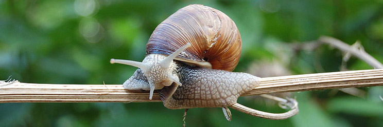
It has long been recognized that not all food eaten by an individual is converted into new animal mass. Consider a stream snail grazing on algae (Figure 1). Only a fraction of the material ingested (I) is assimilated (A) from the digestive tract; the remainder passes out as feces (F). Of the material assimilated, only a fraction contributes to growth of an individual’s mass or to reproduction — both of which ultimately represent production (P). Most of the rest is used for respiration (R). A small portion of energy is lost in excretion, but is usually ignored in such energy budgets. Simple equations are used to illustrate the fate of ingested energy, such as I = R + P + F. Alternatively, production is P = I - F - R.
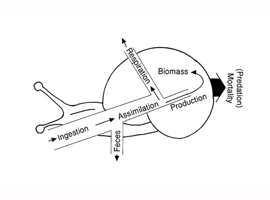
Figure 1: Energy flow diagram of a stream snail population
All flows (ingestion, assimilation, feces, respiration, production, mortality) have units of mg dry mass m-2 day-1). The area occupied by the snail represents biomass (mg dry mass m-2). Production adds to biomass and mortality subtracts from biomass simultaneously. Thus, if production exceeds biomass lost to mortality, biomass will increase. If production is less than biomass lost to mortality, biomass will decline.
Most energy flow diagrams in textbooks show production flowing from one trophic level into another. In reality, however, production is a growth process that must first add to the mass of individuals before it can be consumed in the process of flowing to a predator or the next trophic level (Figure 1). So it is a two-step process: individual growth first creates new population biomass, then some of the biomass flows to the next level as a portion of the individuals consumed by predators.
Widespread appreciation of secondary production arose in the 1960s with the establishment of the International Biological Program (IBP). A major focus of the IBP was to quantify energy flow through trophic levels in various ecosystems, both aquatic and terrestrial, around the world. IBP Handbooks provided the basic methods for estimating production (e.g. Edmondson & Winberg 1971). It was not until the 1970s–1980s that ecologists began fine-tuning methods and addressing questions outside the energy flow paradigm (Benke & Huryn 2010). That is, population production by itself (without respiration, assimilation, etc.) became used as a response variable.
A Simple Method for Measuring Secondary Production
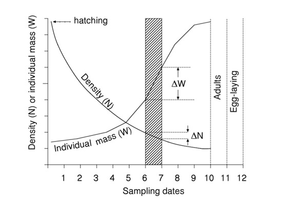
Figure 2: Calculation of secondary production by sampling a cohort
After hatching occurs, the density of a cohort declines, and individuals increase in mass. For any interval of time between sampling dates, such as between 6 and 7, production is easily calculated as the product of the increase in mass (ΔW) and mean density between dates (Ñ).
P= ΣÑΔW
This simple approach accounts for biomass losses due to mortality as well as the accumulation of biomass through individual growth. In this particular example, such as would occur for an insect, somatic production only occurs during the juvenile stages and none during the adult stage. Adults produce eggs, but this contribution to production is often small (depending on the taxon), and would be measured by a different method, if at all. Actual production calculations are easily done in a table or spreadsheet as shown for the larval stages of the dragonfly Epitheca spp. from a pond (Table 1). Production of all time intervals is added to obtain annual production (1927.6 mg m-2 y-1). This approach of estimating cohort production can be applied to other types of life histories, even those in which the juveniles grow within a brood pouch or uterus.
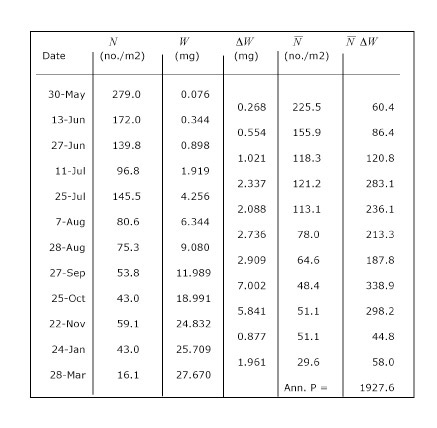
Table 1: Calculation of annual (or cohort) production for the dragonfly Epitheca spp (two indistinguishable species combined) from a South Carolina pond
Production is the sum of the ÑΔW column (modified from Benke 1976).
Production Is Not Just for Energy Flow
Although most ecology texts discuss secondary production only as it applies to ecosystem energy flow studies, many applications in recent decades have been for different purposes, particularly for freshwater benthic invertebrates (Benke & Huryn 2010). Examples of applications addressing both energetic and other ecological questions are briefly described here.
- How can production be used with ecological efficiencies to better understand energy flow? The basic ecological efficiencies are assimilation efficiency (assimilation/ingestion or A/I), net production efficiency (production/assimilation or P/A), and gross production efficiency (production/ingestion or P/I). Calculations of I, A, R, and P are typically done in the laboratory using various methods. Growth of individual mass in the laboratory is used as a surrogate for production in the field. We can calculate that if an herbivore (such as a snail, Figure 1) was found to have an assimilation efficiency of 25% and a net production efficiency of 40%, then its gross production efficiency (A/I x P/A) is only 0.25 x 0.40 = 0.10, or 10%. Thus, if all the organic matter produced by algae was consumed by snails, snail production could only be 10% of algal net production. An obvious lesson learned is that for any plot of land or volume of water, only a small fraction of potential food obtained from autotrophs can be converted to animal production, assuming 100% consumption. With good estimates of both primary and secondary production, and of ecological efficiencies, we can calculate the fraction of primary production actually consumed by grazers. This fraction is not necessarily 100% and can provide considerable insight into top-down effects of animals on their food resource.
- Is a gross production efficiency of 10% realistic for all trophic levels? It appears that great variation occurs, depending on the types of organisms involved. For example, while P/A can be quite high, such as 40% for our snails, P/A is commonly less than 4% in endothermic animals (mammals, birds) which would yield a P/I much lower than 10%. On the other hand, invertebrate predators, such as the dragonfly in Table 1, typically have much higher assimilation efficiencies (70–90%) than herbivores (10–30%). Thus, it is possible that >30% of herbivore production might be translated into predator production (e.g., 0.9 x 0.4 = 0.36). Bruce Wallace and colleagues (1997) actually found that the production of predacious invertebrates was about 36% that of primary consumers in a stream ecosystem over many years, implying that close to 100% of primary consumer production was eaten by predators. In short, while we can generalize about a 10% transfer efficiency, it is actually extremely variable (e.g., Humphreys 1979).
- How is annual production related to mean annual biomass? The answer to this question provides a direct estimate of biomass turnover rates and its relationship to length of life. Studies have shown that if a population has a life span of one year, then the ratio of annual production to mean biomass throughout the year (P/B) is roughly 5 (Waters 1969). Furthermore, the ratio is inversely related to life span. A five-year life span would result in an annual P/B of about 1. A thirty-day life span would result in an annual P/B of about 60. Thus, great variation can occur in annual P/B which represents the rate of biomass turnover: an annual P/B of 30 means that the population replaces its own biomass thirty times over the course of a year through the processes of growth and death.
- How does production vary within a year and what can this tell us? Although typical production studies use annual values, Figure 3 shows weekly production of the dragonfly Epitheca from Table 1 for an entire year, as well as for the other two most productive dragonflies in the pond. Such short-term measurements are obviously more informative than annual values. All species clearly have more production during summer than winter, a reflection of higher growth rates at higher temperatures. Examination of such patterns sometimes suggests niche partitioning along the time dimension among species, but that is not apparent here. Since consumption is directly related to production, however, these temporal patterns suggest much higher predation by dragonflies on their prey (chironomid midges and mayflies) during summer months.
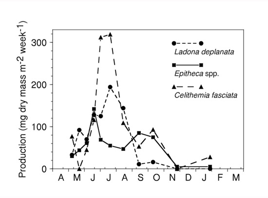 Figure 3: Weekly production of the three major dragonfly taxa throughout a year from a South Carolina pondBased on data from Benke 1976.
 - What is the relative importance of potentially competing species in a community? Production is a particularly useful response variable for this purpose because it is a reflection of a species success and its function (i.e., how much food it consumes and how much food it can potentially contribute to its predators). In the case of the three dragonflies, these species are clearly co-dominant predators in the pond with production ranging from only 1.93 to 2.27 g m-2y-1. These three species were estimated to contribute about 75% of total dragonfly production in the pond, even though there were at least ten other dragonfly species present. Similarly, it becomes possible to compare one population of a species to another of the same species across habitats, communities, or experimental treatments.
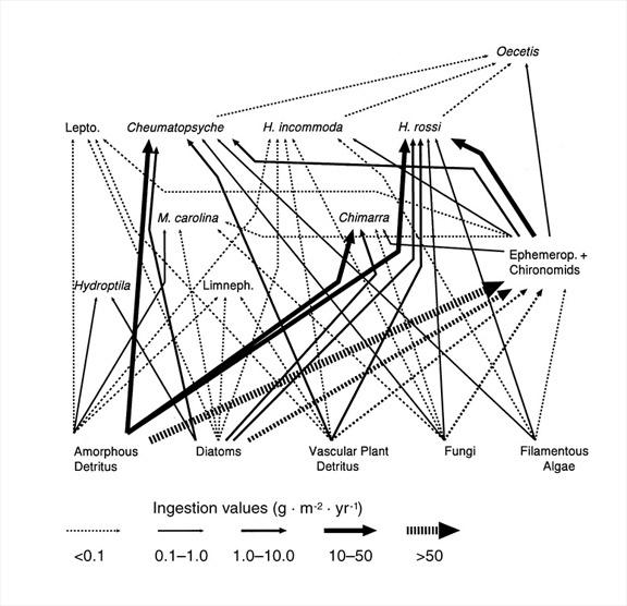
- How can food webs be quantified using production? Species-based food webs are a topic of intense interest in ecology, but there are several ways in which they can be constructed. Bruce Wallace and I developed a method to quantify ingestion flows among populations using a combination of production and gut analyses (Benke & Wallace 1997). In constructing such webs it is necessary to make assumptions of ecological efficiencies from the scientific literature (see 1 and 2 above). Figure 4 shows a partial quantitative flow web focusing on the caddisflies of an aquatic insect assemblage on submerged wood in a river. Note that flows vary by more than 500-fold and that several species consume significant amounts of animal prey. Clearly, these caddisflies do not fall easily into a single trophic level. Such webs are far more detailed than coarse measures of energy flow through trophic levels and far more informative than connectivity webs in which all species-species connections are considered equal.
Figure 4: Quantitative food web for the major caddisfly taxa on submerged wood habitat in a river
Line thickness indicates magnitude of ingestion flows (g dry mass m-2 y-1). The heavier dashed lines are approximations of flows to mayflies (Ephemerop) and midges (Chironomids). Lepto. are members of the caddisfly family Leptoceridae and Limneph. are members of the family Limnephilidae. All other taxa are to genus or species. (Figure from Benke and Wallace 1997)
In summary, secondary production is a comprehensive population variable that incorporates density, biomass, individual growth rates, population death rates, and life spans. It has not only been used in ecosystem energy flow studies, but has addressed a wide variety of ecological questions. It is often superior to density or biomass alone as a response variable because it is a measure of function rather than structure.
References and Recommended Reading
Benke, A. C. Dragonfly production and prey turnover. Ecology 57, 915-927 (1976).
Benke, A. C. Secondary production of aquatic insects. In Ecology of Aquatic Insects. eds. Resh, V. H. & Rosenberg, D. M. (New York: Praeger Publishers, 1984) 289-322.
Benke, A. C. & Huryn, A. D. Secondary production of macroinvertebrates. In Methods in Stream Ecology, 2nd ed. eds. Hauer, F. R. & Lamberti, G. A. (Burlington: Academic Press, 2006) 691-710.
Benke, A. C. & Huryn, A. D. Benthic invertebrate production: facilitating answers to ecological riddles in freshwater ecosystems. Journal of the North American Benthological Society 29, 264-285 (2010).
Benke, A. C. & Wallace, J. B. Trophic basis of production among riverine caddisflies: implications for food web analysis. Ecology 78, 1132-1145 (1997).
Cusson, M. & Bourget, E. Global patterns of macroinvertebrate production in marine benthic habitats. Marine Ecology Progress Series 297, 1-14 (2005).
Edmondson, W. T. & Winberg, G. G., eds. A manual on methods for the assessment of secondary productivity in fresh waters. IBP Handbook No. 17. Oxford, UK: Blackwell Scientific Publications, 1971.
Humphreys, W. F. Production and respiration in animal populations. Journal of Animal Ecology 48, 427-453 (1979).
Huryn, A. D. & Wallace, J. B. Life history and production of stream insects. Annual Review of Entomology 45, 83-110 (2000).
Meyer, C. K., Whiles, M. R. et al. Life history, secondary production, and ecosystem significance of acridid grasshoppers in annual burned and unburned tallgrass prairie. American Entomologist 48, 52-61 (2002).
Odum, E. P. Fundamentals of Ecology, 2nd edition. Philadelphia, PA: W. B. Saunders, 1971.
Whalen, J. K, & Parmelee, R. W. Earthworm secondary production and N flux in agroecoysystems: a comparison of two approaches. Oecologia (Berlin) 124, 561-573 (2000).
Wallace, J. B., Eggert, S. L. et al. Multiple trophic levels of a forest stream linked to terrestrial litter inputs. Science 277, 102-104 (1997).
Wallace, J. B. & O'Hop, J. Life on a fast pad: waterlily leaf beetle impact on water lilies. Ecology 66, 1534-1544 (1985).
Waters, T. F. The turnover ratio in production ecology of freshwater invertebrates. American Naturalist 103, 173-185 (1969).
Waters, T. F. Secondary production in inland waters. Advances in Ecological Research 10, 91-64 (1977).